In Spring 2023, I took the course CSE 168 (Computer Graphics II: Rendering) with Professor Tzumao Li. It was a really fun course that focused on raytracing as the intersection of a wide range of fields, including physics, statistics, signal processing, high-performance computing, and even art. In fact, to paraphrase the professor, computer graphics research/development is an art as much as a science because, while there are still tradeoffs to analyze and metrics to optimize, the ultimate goal is just to figure out what makes things look good.
Each homework assignment in the course built up one core part of a raytracing program using C++, which was written to run on the CPU (and parallelized with OpenMP). Below are the custom scenes that I designed and rendered with my code to showcase its features. All 3D models were provided as part of the course materials except for the Geisel Library models, which I created.
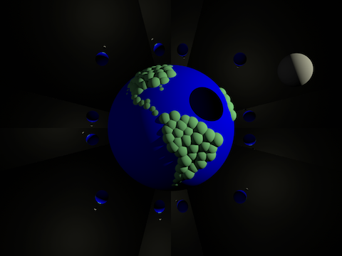
In the first assignment, we implemented basic raytracing functionality, sphere objects, diffuse and mirror materials, and point lights.
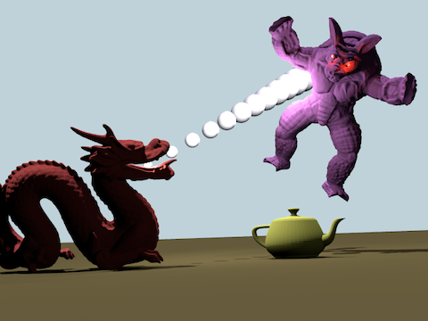
In the second assignment, we implemented triangle meshes and the bounding volume hierarchy acceleration structure to allow more interesting, detailed objects. On the left, for example, is the Stanford Dragon model with hundreds of thousands of triangles.
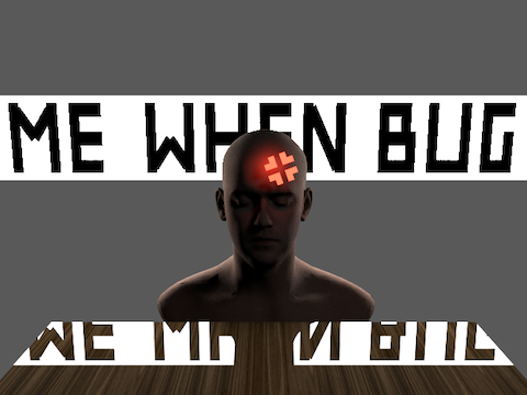
In the third assignment, we implemented a plastic/clearcoat material, texture mapping, and area lights. Note the glow of the red lights on the face and the rim lighting on the shoulders. The head model is a textured 3D scan by Lee Perry-Smith.
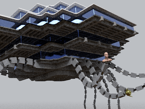
In the fourth assignment, we implemented path tracing and multiple importance sampling to achieve indirect illumination. Note the (rather noisy) indirect lighting from the blue windows onto the gray roofs and from the brown floor onto the underside of the robot. The robot model was created by me based on UCSD's Geisel Library.

In the final project, we implemented additional features of our choosing in the raytracing program. I first added a glass material so I could produce this image of Geisel Library in a snow globe, rendered at 512 samples per pixel in about 300 seconds. Note the significant amount of bright pixels ("fireflies") in most regions, especially the bottom half of the globe. These are an expected result of our Monte Carlo sampling methods, but are typically undesirable. The goal of my project was to try to remove them.

The main feature of my project was adaptive sampling and denoising, based on a 2012 paper by Professor Li. This version of the above image was rendered with 8 iterations of adaptive sampling at an average of about 32 samples per pixel in each iteration, taking about 310 seconds. Adaptive sampling sends more samples to pixels with high variance, which greatly reduced the fireflies in the image. However, the overall image has slightly more noise due to the lower total number of samples.
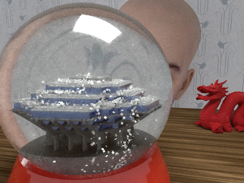
The other big part of my project was denoising, based on the same paper as above. This version is the result of the denoising algorithm run on the previous image, which took about 320 seconds total. Much of the noise is smoothed out, while edges and important features are preserved like most refractions in the globe, the reflections around its edges and base, the shadows on the dragon, and the pattern of the wallpaper. However, there still weren't quite enough samples to capture the refraction of the wallpaper's thin lines in the globe, so they look a bit fuzzy. Overall, glass and other reflective materials are a pretty difficult case for raytracing and denoising because they cause much greater variance than diffuse materials, but this algorithm seems to have done alright.
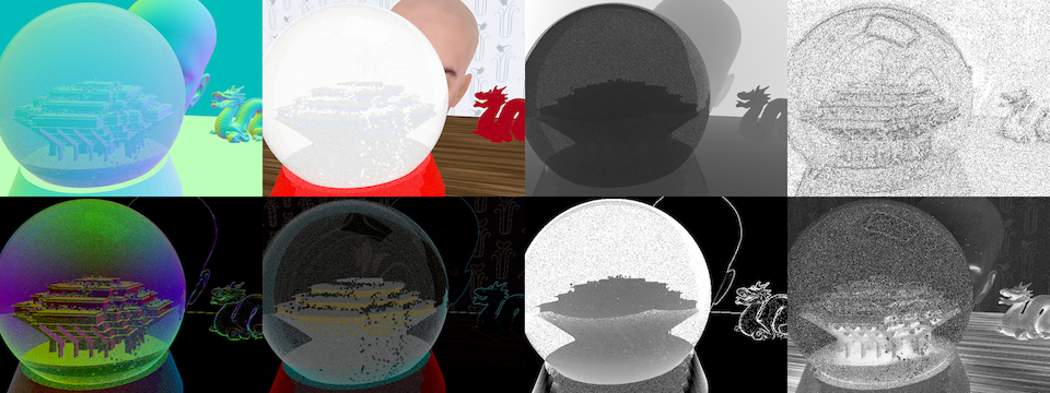
Finally, denoising computer-generated images can often be easier than denoising real photographs because we can obtain additional information about the scene besides color. Here are the extra features from the above renders that I used for the adaptive sampling and denoising algorithm. From left to right: surface normals/variance, texture albedo/variance, intersection depth/variance, and outputs from the algorithm.